|
home | what's new | other sites | contact | about |
|||
|
Word Gems exploring self-realization, sacred personhood, and full humanity
Quantum Mechanics
return to "Quantum Mechanics" main-page
transcript of Dr. Brian Greene's "Your Daily Equation #21" featuring Bell's Theorem (see youtube)
Hey, everyone. Welcome to this next episode of Your Daily Equation. And today, I’m going to take up a result that some physicists, some commentators have described as the most profound result in theoretical and experimental physics. I’m not sure I would agree with it as the most profound, but without a doubt, it ranks among the top few of the most remarkable, most surprising insights that have emerged say in the last 100-150 years. So it’s well worth spending a little time thinking about it. And the topic that we’re focusing upon is the possibility that our world allows for influences that are nonlocal. What does that mean, a nonlocal influence? What’s a local influence? Well, that’s an ordinary influence. You do something, whatever, you snap your fingers, you clap your hands, you push something, you move something around, and the influence that you exert manifests in your local environment. It’s unusual to imagine that you could, say, punch your fist forward and like hit somebody in the back of the head or on the nose on the other side of the country. I don’t sort of like that violent metaphor, but you sort of get the gist. What you do according to logical reasoning, what you do according to everyday experience, what you do according to the laws of physics as we thought we understood them prior to what I’m going to talk about here today, what you do here influences things here. It doesn’t influence things instantaneously or immediately some place far away from here. So locality is you exert influence, it effects your local environment. Nonlocality is the possibility that you exert some kind of influence and it affects something far away. And it was the insight of a variety of individuals. We’ll talk about a number of them today, but let me bring them up on the screen. Albert Einstein right here played an absolutely essential role in the story that I’m going to describe here because it was his insight together with two colleagues, I’ll show you them in a moment, Podolsky and Rosen, that came up with an idea that ultimately rippled through our understanding of physics, giving us a radically different picture than even Albert Einstein would have anticipated. And this relies upon a variety of ideas having to do with quantum mechanics, quantum entanglement. The culminating effort in this direction emerges with this guy over here, who among physicists is extraordinarily well-known. For the general public, less well-known.
This is John Bell, an Irish physicist, who, as we will see, was able to take a completely abstract theoretical idea, almost a metaphysical idea, at least it seemed metaphysical in the sense that it didn’t seem to have any experimental consequences that Einstein and his colleagues came up with, and Bell was able to show that Einstein’s idea was not metaphysics. That Einstein’s idea was physics, which meant Einstein’s idea could be tested. Indeed, as we’ll see, he wrote down the test, and later on physicists came along and carried out that test to profound effect. Okay. So here are the three main culprits in the story, Einstein, Boris Podolsky and Nathan Rosen. And it was in 1935 that they wrote this paper over here. If you’ve been following the series, you’ll note that in the episode on quantum entanglement… I don’t know what episode it was. You don’t have to have watched that episode to understand the discussion here today, but it would help if you looked at that. So in that episode, I described the basic idea of entanglement and the basic conclusion of the paper that Einstein and his colleagues wrote here, but I’ll remind you of that again. And again, the overarching implication or the overarching message of Einstein’s paper with his two colleagues was not that quantum mechanics was wrong. So this headline in The New York Times really is spot on, Scientist and Two Colleagues Find It Is Not ‘Complete’ Even Though ‘Correct’. So Einstein and Podolsky and Rosen were never saying that quantum mechanics is wrong in the sense that it makes predictions that are in conflict with observation or experiment. What they were saying instead was the view of reality that quantum mechanics puts forward is an incomplete description of reality. And Einstein and his colleagues were arguing that there has to be a deeper description. Even though they were unable to give that deeper description, they believed that in this paper they had established that there was a deeper description waiting to be found. And their analysis relied on this idea of quantum entanglement, which pictorially is this idea that you can have two particles that can be widely separated, and yet there’s still a kind of quantum mechanical thread, an invisible thread. I showed here in yellow just to sort of give it a little visualization. But it’s as if there’s an invisible quantum mechanical connection that links these two particles regardless of how far apart they are and allows it to be the case. According to standard quantum mechanics that if you do something to one of these particles, say the one on the right, it can have an immediate influence on a measurement on the particle on the left of the image, even though they might be miles, kilometers, light years apart. That is very strange, and this is why Einstein called this spooky, right? It was a spooky implication of bread and butter quantum mechanics that you could set up two particles in this manner such that you perform a measurement on one of those particles and it immediately, instantaneously has an impact on a measurement undertaken on the partner particle regardless of how far apart they are. I mean, that’s crazy sounding talk, right? But yet, that’s what standard quantum mechanics seemed to be implying. And Einstein and his colleagues came along and said, “We don’t buy that. We believe there’s a different picture,” and I’ll show you what the picture is that Einstein, Podolsky and Rosen put forward. And that picture is ultimately what John Bell analyzed and showed that that new picture could actually be subject to experimental tests. And as we’ll see, the way in which Einstein and his colleagues envisioned the world behaving is not actually born out by the experiment. It’s not fully refute it as some say, and I’m going to come to that subtly toward the very end. But the image that Einstein had of a world in which influences would be local seems not to be our reality. It seems to be the case. And I’m hedging my description only because at the end I’ll describe one or two potential loopholes in this conclusion. But the most straightforward reading of the discussion that I’m going to have here now is that our quantum mechanical world does allow this kind of nonlocality, does allow a measurement in one location to have an influence on a measurement taking place at a distant location regardless of how far apart they are. All right. So I’m not going to follow the precise way in which Einstein and his colleagues came to this conclusion. Instead, I’m going to use the same kind of example that I used in the discussion earlier of quantum entanglement, that earlier episode, which makes use of this property of particles called spin, quantum mechanical spin. Now, not everybody’s familiar with the quantum mechanical spin. Roughly speaking, for the purposes that we have at hand here, you can think about it as follows. Particles have a quality that allows you to think about them as if they’re spinning around like a top. And any given species of particle has a fixed amount of this quantum mechanical spin. The Higgs boson was so special because it has none of this quantum mechanical spin. It’s the first particle that we’ve ever encountered that doesn’t have a certain of spin. Well, it does a certain amount. It’s zero in that particular case, but electrons and the quarks and the familiar matter particles have an amount of quantum mechanical spin called spin 1/2. All that means pictorially which is fine for what we’re discussing here is this. So you can have a particle and I kind of hope you can see this. This particle is actually spinning around. Get close to your screen if you don’t see it. Yeah, I think you can probably see it. So it’s spinning around. In this particular case, it’s going in a clockwise orientation. The particle can also spin around this axis the other direction. The same amount, roughly speaking, the same speed of spin, if you will. And we have an arrow that we could point directly in the direction of the spin as in this particular case here with the orange arrow, or the other direction we could have this purple arrow going say in this counterclockwise direction. It’s really awkward to try to have arrows that spin around with the particle, so we use different notation. So for this case, instead of having the arrow going around with the particle, we say that the particle is spinning up, which is just the right hand rule. Take your fingers, you curl it in the direction of the spin, and your thumb points in the direction that we use to describe that kind of spinning motion. So in this case, counterclockwise spinning up and the opposite would be spinning down. And again, you have to get really close to see it, but that particle is spinning around in this clockwise direction, which by this right hand rule would be spinning down. Now, the weirdness of quantum mechanics really come to the fore when we realize that quantum mechanics allows a particle to be in kind of a fuzzy mixture of both spinning up and spinning down at the same time. And it’s hard to show that pictorially, but take a look at this, right? This is not a really good depiction, but it gives you rough sense that it’s kind of up and down. The problem with this imagery is at any given moment, if I was to stop this animation, the arrow would be up or it would be down, which would mean that at a given moment, it had one or the other spin. That’s not what quantum mechanics tells us. Quantum mechanics tells us that the particle is in a mixture of both spins at the same time. So I can’t really depict that, but this is sort of not a bad visual image, visual metaphor to have in mind. And only when you measure the particle does it snap to attention and acquire a single definite spin. In this case, it snapped to attention spinning in the upward direction. But if this is a 50-50 mixture, half probability of up, half probability of down, then you know if I measured again, it could be up or down, 50-50 chance. And in this particular animation, it turned out that that second measurement gives this particle spinning in the downward direction. So it’s weird. Very strange. Quantum mechanics allowing this sort of fuzzy, nebulous reality until a measurement or an interaction takes place which forces that reality to ante up and choose one or the other outcome. In this particular case, there are only two possible outcomes. The particle chooses one or the other only when the particle is confronted by a measurement or confronted by an appropriate interaction that disambiguates this blending of possibilities, which is the reality prior to that interaction. So totally strange, but this is the standard part of quantum mechanics. It’s got a weirdness in its own right, but now we go further. And the weirdness of quantum entanglement as applied to this particular example of quantum mechanically spinning particles is this. According to quantum mechanics, you can set up a situation where you have two particles, each of which is in this fuzzy mixture of spinning up and down at the same time. But you can set it up so that their spins are correlated so that they’re both in a 50-50 mixture up and down, but the spin of one is opposite to the spin of the other. In the sense that if you were to set up this situation, they’re both of 50 up, 50 down, let’s say you go to the particle on the right. You measure it. It snaps out of the haze, purple pointing up, and the particle on the left, or at least my left, is pointing down. I always get confused if your left and my left will be the same. So I hope that what I’m calling right and left is not reversed, but be that as it may. The purple one is spinning up and the orange one is spinning down. And the curious feature of this is I only interacted with the purple particle, at least the one that turned out to be purple, and it forced the other particle to disambiguate and spin down once the one that turned out to be spinning acquired that definite spin. That’s the weirdness of quantum entanglement because these two particles could be arbitrarily far apart. And an image that makes this a little bit more dramatic and it’s schematic, but it’s more energetic, if you will, here are two entangled particles in this 50-50 mixture spinning up and spinning down. I go to the particle on the right, and I measure it. It spins down. Immediately the one on the left snaps out of the haze and spins up. Again, I can do this again. They’re 50-50 mixture up and down. Let’s say I go to the part on the left, and I measure it and snaps out of the haze spinning down. The one on the right will snap out of the haze instantaneously spinning the opposite orientation. And that is the weirdness of quantum entanglement and that’s the spookiness of it, right? I mean, how could it be that you measure one and it affects the other? So what does Einstein do? Well, let me show you what he does in the context of taking these abstract examples of spinning particles. Let me put them into more of a laboratory setting. Okay? So in a laboratory setting, we can imagine that we have, say, a couple of detectors, and one detector on the right, one detector on the left, and in the middle is a device, if you will, that will send out particles that are entangled.
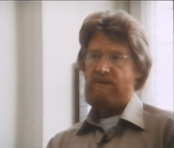
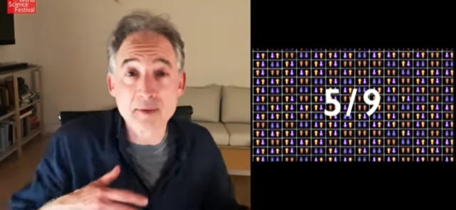
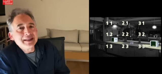
So this device in the middle creates entangled particles and it creates them in just the way that we’ve been describing, one up, one down, the other up, the other down, and so forth. And these detectors are able to measure the spins of the particles. So the example that I was just showing you a second ago in this language would look like this. Two particles say are emitted from the center device. They’re both in the mixture up and down, and then they get measured on the left and the right. And when they’re measured, one is up, one is down, or in the reverse case, the other is down, the other is up, and so forth. But the weirdness, the spookiness is that they’re in a fuzzy mixture, and yet upon measurement, they both disambiguate. They both choose a definite reality. Even though they’re far apart, they’re able to correlate the outcomes. That’s the weirdness. So far apart and yet they never get it wrong. When one’s up, the other is down. When one’s down, the other is up. Amazing. Right. So what does Einstein say to this? He says, “Look.” He says, “That’s two damn spooky for me.” He says, “I think what’s really going on here is not that these particles are in this fuzzy mixture of up and down until they get to the detectors, and only upon measurement do they snap out to be one way or the other.” He says, “That would require some spooky crosstalk between them, some spooky conversation between these widely separated particles.” He says, “The world doesn’t work that way.” So he says, “I have got a much simpler explanation for what’s really going on here.” He says, “If a detector measures a particle and finds it spinning up, then it always was spinning up. It was never in this fuzzy mixture of spinning up and down as the math of quantum mechanics tells us.” He says the math of quantum mechanics is simply unable to get at the full and complete description of reality. And that’s why it seems to us by staring that the equations that a particle is in a fuzzy mixture of up and down until measurement. When in reality, it always was up or down from the get-go. And then to explain how when this one’s down, this one’s up, very simply, this was always down and this was always up, and that’s how they were from the get-go. And these detectors simply revealed the definite spin that they already had. So pictorially it’d be like this. We have here the spins of the particles coming out, and they’re definite from the get-go, according to Einstein, Podolsky and Rosen. The one on the right, at least my right, is spinning up. The one on the left is spinning down. And that’s all there is to it. So of course, as they race toward their two detectors, they maintain those spins and the detectors reveal those spins. So Einstein says, “Here is what’s really going on. Particles have definite properties.” Even though quantum mechanics can’t give us those definite properties, quantum mechanics only gives us probabilities of those definite properties, but definite properties the particles have and they’re opposite to each other, on the left and the right. And therefore, it’s no surprise that the measurements always yield this perfect anti-correlation, one is up, the other is down, one is down and the other is up. Nothing spooky at all in this Einsteinian, Podolskian, Rosean description of the true underlying reality. So this is what The New York Times meant when they said that Einstein, Podolsky and Rosen were not saying that quantum mechanics is wrong. They’re saying it’s incomplete. They’re saying that sure, the predictions of quantum mechanics, spot on accurate, but the true picture of reality that underlies the mathematical description is quite different, they are claiming, form the reality that’s manifest in the quantum mechanical mathematics. According to quantum mechanics, particles can be in this mixture. And then measured, they snap out of the haze. Einstein says, “No, no, no, no. They always had a definite spin. It’s just that your incomplete quantum mathematics is unable to tell us that definite disposition. And because your theory is incomplete, it’s reduced to giving probabilistic descriptions of a reality, but that’s only a description. That’s not how reality actually works.” Now, when Einstein came forward with this idea, there is definitely some… How should I say it? Well, there was concern that Einstein maybe was pointing out a failing of quantum mechanics. Maybe Einstein was right. But then people began to think about it more fully and they began to realize or at least they began to think that they realized that Einstein’s view of reality could never be tested, fundamentally couldn’t be tested, right? I mean, this guy over here, Wolfgang Pauli, he said that Einstein and Podolsky, Rosen’s view of reality was no better than the ancient question of how many angels can dance on the head of a pin? It was something that was untestable. Now, why would be it untestable? Well, you see, Einstein is saying that before you measure the particle, it has a definite spin, whereas quantum mechanics says it’s in a mixture, right? But how do you verify that picture without measuring the particle? The only way you can learn the disposition of the particle is by measuring it. But after measurement, Einstein agrees that it will a definite value, say up or down, and quantum mechanics agrees that it will have a definite value up or down. They only differ, these two views of reality only differ from each other prior to the measurement. How can you ever test something that’s prior to the measurement? It’s as if I said to you, hey, guys, did you know that I actually have pink hair? But anytime you look at me, my hair turns white or gray, whatever color my hair is, right? My statement that I have pink hair when you’re not looking is fundamentally untestable because to test it, you need to look. But I’m stipulating that when you look, my hair is no longer pink. So Pauli makes the analogy to angels dancing on the head of a pin. Niels Bohr, who was Einstein’s deep partner in trying to understand the fundamental laws of physics, Bohr’s view was he said, “Look, it is a mistake to think that we physicists are in the business of trying to find the true nature of reality.” “Nonsense,” Bohr says. “We are in the business of trying to find the equations that will make accurate predictions for the results of measurements. And if you try to think that we physicists are doing anything more than that, you’re going to run into problems.” And that he says is what Einstein has run into. He basically says, “In the end, if there’s no experimental difference between the Einsteinian view of the underlying reality and the quantum mechanical view of the underlying reality, then we’re not talking physics any longer.” So Einstein passes away in 1955. Bohr passes away in 1962. And this issue of what the true nature of the world is, is the world in a fuzzy probabilistic haze until measured or until there’s a suitable interaction, or is the world actually definite and your measurements just reveal that definite reality? Which of those pictures is correct? People basically don’t pay a lot of attention to the issue for a period of time. Because they think it’s fundamentally untestable, fundamentally not physics, fundamentally perhaps philosophy. I don’t mean that in the derogatory way. I mean more of a philosophical view of how the world is opposed to a physicist’s view of the things that we can measure in the world. And that’s where this guy I mentioned early on in this episode, John Stewart Bell, comes into the story. Because in 1964, he writes a paper. I’ll show you that paper in just a moment. He writes a paper that shows the Einstein view of reality is testable. Pauli was wrong. It’s not about angels dancing on the head of a pin. Bell surprisingly shows that Einstein’s view of a world in which qualities are always definite, that yields a measurable difference, an experimentally distinct prediction from the quantum mechanical prediction. Now, how does he do this? Well, I’m going to focus on the little example that we’ve been looking at about particle spin. I mean, the paper that Bell writes is much more general than that, but let’s just try to get at the heart of the manner. What is the essential new idea that Bell introduces? He says, “Look, let me just imagine doing that laboratory experiment with the spinning particles, with the two detectors in the opposite ends of the laboratory bench, but let me imagine that I went to the physics supply store and I got some better detectors, upgraded detectors. Imagine that the detectors don’t just measure the spin along one axis, the vertical axis that we were looking at. Imagine that it can measure that particle spin about three different axes, axis one, axis two, and axis three.” Now, exactly what those axes are does matter to the mathematical version of the argument that I’m about to give you. You don’t really need to know that because I’m going to focus sort of at a higher level. We will do the mathematical analysis, but we won’t get into that level of detail. But just in case you’re interested, the three axes that Bell envisions are axes that are at 120 degrees relative to one another. This axis, that axis… Like a peace sign. That axis, this axis, and this axis. And so what this detector does is when the particle comes in, you the user, the experimenter, pick one of the three axes while the particle is say in flight. You pick axis one or two or three, and the outcome will be the measurement of the particle spin along that axis. Now, the weirdness of bread and butter quantum mechanics that nobody is questioning is that the result of that measurement will always be spin up or spin down along that axis. Now, I’m not going to distinguish in the read out the different orientations. It’ll always show up or down, but you take it to mean that it’s up or down along axis one if I pick one, up and down along axis two if I pick setting two on the detector. Similarly, up or down along axis three if I choose setting number three. And again, just so it’s clear, here is Bell’s paper which I can just thumb through it again. It’s not long. And you see that there’s more general mathematical analysis that you see in this, but it’s nothing more than basic quantum mechanics, linear algebra. On this right hand page toward the bottom, a little bit of calculus. But that’s it, right? That’s the end of this paper, which gives us in the end as we will see a shocking insight, shocking conclusion. But the version of understanding this at a pedagogical level that I will follow, following this example of the particle spins, I learned from this guy over here, David Mermin. I was a professor at Cornell in the 1990s. David Mermin has been at Cornell for a very long time. I think he may be retired now, and he just has this spectacular knack for drilling down and really finding the heart of an argument. Now, I remember, I went to a colloquium at Cornell where David Mermin was explaining Bell’s ideas. And I sort of heard of Bell’s ideas at that time. Look, as a faculty member at that time, I sort of knew about Bell’s ideas, but I didn’t really know about Bell’s ideas. And after this colloquium of David Mermin’s, I was just like walking around in kind of state of shock when I finally understood in an intuitive way, that I will explain right now, what John Bell was telling us. Okay. So let me show you then how the argument goes in this particular version that David Mermin gives us. So here’s our detector. We can choose axis one, axis two, axis two, and each of these detectors are in this configuration. And now, I should say, when a particle pair is emitted by this particle creation in the center there, it sends the particles out left and right. Now the particles have to have definite spins along all three of the possible axes, according to Albert Einstein. Einstein says again, particles have definite features. When you measure something, you measure something that’s already there. So if we’re measuring the particle spins along axis one, then the particle better have a definite value of the spin along axis one. And you see it right here, the left particle is spinning up along axis one and the right… Again, they’re completely anti-correlated. That’s the nature of this entangled state. But you see particle one, the particle on the left along the first axis is spinning up, particle number two along the first axis is spinning down. Similarly, the particle on my left along the second axis, you got the purple pointing down. The corresponding measurement on its entangled partner particle on the right, the middle arrow is spinning up. And finally, you see that the third arrow on the left particle is spinning up, the third arrow on the right is spinning down. So according to Einstein and colleagues, this is the true nature of the underlying reality. It’s none of this business along these axes. And now the explanation for the results in this view of reality would be completely clear. So let’s imagine we run some experiments. Let’s say we pick axis one for the detector on the left and the right. That means the first arrow for each of the entangled particles dictates the outcome, and you see the one on the left is spinning up and the one on the right is spinning down. Now, if I pick the second axis for both of these, it’s the second arrow and it triples that matter, so you got spinning down on the left, spinning up on the right. And for good measure, let’s set the detector to be axis three and it’s the third arrows of each of these triplets that matters, spinning up on the left, spinning down on the right. And the detector simply reveal the underlying quality of the particle that Einstein and his colleagues say is truly the nature of the deep description of reality. Now, so far you say, okay, so John Bell doesn’t seem to have done very much. We’re just doing the same kind of experiment, but now we just have the choice of picking the axes. But here’s the thing, in the three examples that I just gave you, I happen to choose the axis on the left detector and the right detector to be the same. Left was one, right was one. Left was two, right was two. Left was three, right was three. But we don’t have to choose. This is the freedom of this new scenario. We don’t have to choose the axis to be the same. I could choose different axis for each of the two detectors. Like I could choose on the left, maybe I choose setting number two. And on the right I choose one, or on the left I choose three, or on the right I choose two, and so forth, right? And with this newfound freedom to have different settings on the two detectors, we can now get results quite different from what we’ve gotten so far. So far all of our results were this one’s up, this one’s down, this one’s down, this one’s up. But now in this case, we can get situations where both are up and both are down [because they can represent spins on different axes]. And that’s important as we’ll see. So let me take a look at that. So let’s do an example. Here’s a case where you got three on the left, two on the right in terms of the detector settings. And what’s the result going to be? Well, look, the three on the left means it’s the third arrow and the triple on the left is pointing up. The two on the right means it’s the middle arrow for the particle on the right. It’s also pointing up. And therefore, your result will be up and up. Hmm, a new result, new kind of result that we didn’t see before. Let me do another example. Let’s say I choose my detector settings to be two on the left and one on the right. That means it’s the middle arrow on the left that’s relevant because it’s the second axis. It’s the first arrow on the right that’s relevant because I chose that detector to measure along the first of the three possible axes. So that means I’m going to get two on the left which is spinning down and one on the right that’s also spinning down, so I should get down-down. And what do we get? Down-down. The detectors work. They do exactly what they are meant to do. And so what this means is if I then run many, many versions of this experiment, particle pair after particle pair going toward the detectors, as they’re in flight saying, “I have a team of physicists at the left detector, a team of physicists at the right detector,” and they’re say randomly picking the axes, what will happen is we’ll get a whole slew of different answers. Sometimes it’ll be up and down. Sometimes it’ll be down and up. Sometimes it’ll be up and down. Sometimes it’ll both be the same. In that case, it was down-down. So you could then imagine doing this experiment over and over and over again and just collecting a whole lot of data for the outcomes. And here’s where Bell’s insight comes to the fore. Bell argues, and I’ll show you the argument, in this case right now, Bell argues that if you do this experiment many, many, many times, randomly choosing the detector settings on each run of the experiment, he argues that the results in which they are anti-correlated, up and down, at least five-ninths of the time the particles have to have that disposition as opposed to this or this.
A prediction that emerges from this view of reality, that particles have definite spins along all of these axes that are being measured. Let me show you how the argument goes. It’s quite simple. So if you think about it, there are obviously nine combinations of possible detector settings. One on the left, one on the right. One the left, two on the right. One in three. Two in one. You got three possibilities for the left detector, three for the right detector. Three times three is nine. So there are nine possible joint settings of these two detectors.
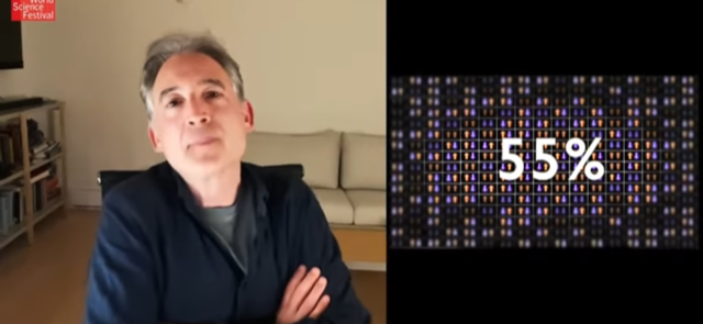
And what I want to do following David Mermin’s version of John Bell, I want to analyze the results that we will get for one particular value of the spin of the two entangled particles. So let’s just look at an example of that here. So imagine that my particle is up-down-up on the left, down-up-down on the right. Now, I’m just going to go detector setting by detector setting to see what I would get. So if the detector settings are one and one, first axis in both of the detectors, then it’s the first arrow in each of the triples that matter, so I get up and down. What if the detector setting was say one on the left and two on the right? Then it’s the first arrow on the left and it’s the second arrow on the right. That’s an up-up. And now you see I can just continue to fill in the table. I’ve got the data in front of me. So if it was two and two, it’ll be the second arrow. That’d be down and up. Two and three, it would be down and down because they now have the down arrow from the particle on the right and so forth. All right. So I continue to fill in the table. Now let me look at the number of outcomes in which the spins are opposite to each other. I’m just going to highlight those so we have them up on the screen, and there you have them. Those are the only ones in which they’re opposite, and we got one, two, three, four, five. Five out of nine of the outcomes have the spins pointing in opposite directions. Okay. That was just one example though. Let me do another example for you. This was an example where particle on the left was up-down-up, particle on the right, the entangled partner was down-up-down. Let’s look at another possibility. Let’s just, for instance, look at a particle on the left hand side where it’s up-up-down, and therefore, down-down-up. Now, as you can see, it’s the same basic analysis, just the results would be shifted around a little. But so I fill in the table just so you can sort of see it. Again, let me focus on those that have opposite spins, which results have opposite spins. And again, one, two, three, four, five out of the nine possible outcomes have the spins being opposite. Now, you might say, well, yeah, you’re only looking at very special cases. But if you have two particles and three axes, then at least two of the spin directions have got to be the same. There are only two possible spins, up or down. You got three possible axes. So you’re going to have two that are the same at least. The only situation that’s fundamentally different from the example that I’ve been looking at here is a case when all of the spins are the same. So let’s look at that case. Imagine on the left particle you have up-up-up, on the right particle you’ve got down-down-down. Now, every outcome along every measurement combination of the axis will give opposite answers. So in this case, you’ll have nine out of nine giving opposite spin results for these nine possible measurements. So it’s five out of nine when all the spins along all three axes are not the same. It’s nine out of nine when they are the same. Therefore, if you imagine running this experiment over and over and over again where you’re just looking at random entangled particles with random detector settings over a huge number of runs of this experiment, at least five-ninths of these results will have opposite spins on the left and the right. At least that's because some of them will have it nine-ninths of the time. So on average, it’s at least 55% of the time you will get opposite spin results.
That is a prediction of the Einsteinian view of the world, that particles have definite spins prior to them being measured. And here’s the thing, you can now test this result. You can do the experiment. There is nothing really Gadonkin-like. These aren’t thought experiments. I mean, when Bell first wrote this down, he knew that in principle you could undertake these measurements. They really weren’t undertaken fully until the late ’70s, early ’80s. They’ve been refined ever since and here is what happens. When you actually do this experiment, you do not get opposite spins five-ninths of the time. You get opposite spins less than five-ninths of the time. In fact, you get opposite spins 50% of the time, not 55% of the time. And therefore, Einstein’s view of the world is in conflict not with our intuition, not with our desire for how the world should be, it’s in conflict with actual experiments that are delineating how the world is. And I should point out the result that you do get from the experiments agrees with the calculation that comes out of standard quantum mechanics. Standard quantum mechanics without this idea that particles have definite features, that particles truly are in this fuzzy mixture, spinning up and spinning down at the same time, it agrees with the experiment, but Einstein, Podolsky and Rosen’s version of reality does not. Now, what are we to make of this? Well, you might immediately conclude that Einstein’s view that particles have definite features is what’s being ruled out here. And based on how I’ve described things, I don’t blame you for thinking that way. But let me now take you back through the chain of reasoning. Einstein said, “The world is not spooky. You don’t have an influence here affecting something else over there.” And in order to get rid of spooky action, he envisioned that particles had definite features. So the whole point of the Einstein-Podolsky-Rosen view of reality is to get rid of spooky action, to get rid of nonlocality by saying that the particles don’t have to correlate their behaviors over long distances. They already have definite features, and the detectors are simply revealing those features. So Einstein is really assuming that the world is local and that the world has these qualities, hidden variables it’s often called, these hidden qualities, these definite features even they may be beyond our ability to know about those definite features until they are measured. So that view of reality is being wiped out by these measurements. And so what we’re really learning is the world cannot be local and have these hidden qualities. Now, it cannot be local and have these hidden qualities. But what that’s telling us therefore is that in principle, it could be nonlocal and have these hidden qualities. That’s not ruled out, or it can simply be nonlocal and not have hidden qualities, which is the approach that standard quantum mechanics takes. But the bottom line is what’s really being ruled out by this whole analysis is that the world is local. We’re learning that these particles behaving like this and like this are making use of a nonlocal connection in the manner that standard quantum mechanics shows should be there. So that is the import of this whole analysis of Einstein, Podolsky, Rosen, John Bell. It’s to come to a conclusion that this vision of the world that comes down to us from Isaac Newton that the world should be local, we learned that that picture runs afoul of the quantum mechanical measurements, measurements of quantum mechanical systems established. That picture is ruled out. The world has nonlocal qualities. Now, I said that with a certain degree of firmness, and now I just want to take a baby step backward because it’s very hard in physics to have fully airtight conclusions. And it’s always a matter of what assumptions you’re making, what paradigm within which you’re working. And as I’ve mentioned a few times in these episodes, quantum mechanics, many of us believe, is not yet a subject in which every T has been crossed and every I has been dotted. There is this issue of the quantum measurement problem, and measurement is all part of the story. What’s the quantum measurement problem? We don’t know how. Even in standard quantum mechanics, quantum mechanics does not tell us how the world transitions from a fuzzy mixture of up and down or a fuzzy mixture of particle being at various potential locations to the single definite reality upon measurement. We don’t know how that happens. And without knowing how that happens, there are potential loopholes to any conclusions that we draw. For instance, there is an approach to quantum mechanics called the many-worlds interpretations of quantum mechanics, and it highlights in essence a third hidden assumption behind everything that we are doing here. Take the Einsteinian view of the world. Einstein is saying the world is local, assumption number one. The world therefore has hidden properties in order to explain long distance correlations. Number three, Einstein is also assuming that when you undertake a measurement, it yields one unique answer. We are assuming that when these particles go to these detectors, the detectors are yielding one answer, up or down. The many-worlds approach challenges that. The many worlds approach says, “Mm-hmm (negative). If the particles in this mixture of up and down, then when it’s measured, you get up in one universe and down in another universe.” You get both answers. If you look at the totality of this larger reality that encompasses all of the universes. And therefore, that’s another way out from the conclusions of this John Bell theoretical result together with the experimental measurements. You could in principle have a universe that’s local, doesn’t have these definite qualities, these hidden variables, these hidden qualities, and scoots around the incompatibility with the experimental measurements by saying measurements don’t have unique outcomes. That is another way to violate the conclusion. And in that way, be compatible with the experimental observations. Putting that to the side, so that’s an interesting possibility, maybe I’ll talk about many-worlds in a subsequent discussion. Allow me to put many-worlds to the side. I mean, that’s so far out in our view of reality. That so radically changes our description of the world that I would not consider that in some sense as restoring us to a more familiar view of the world. That’s even more extreme, if you will, than the nonlocality interpretation. So let me just put that one to the side for a second. So putting it to the side, we are led to the conclusion that the world is not local, that the world allows these nonlocal influence. You do something here and it can affect the outcome of a measurement over there, and this is now coming not from pure theorizing. This is coming from a blending of theoretical insights that start with Einstein, Podolsky and Rosen. People think that there’s no experimental consequence to this view of the world, that it’s local and particles have definite qualities. People think that it’s metaphysics. John Bell comes along and shows us that it’s not metaphysics. And others come along, Clauser, Espey, and others, they do these measurements and they show that Einstein’s view of the world is not compatible with the observations, and something’s got to give. And at least in the traditional description putting many-worlds to the side, the thing that has to give is that the world is local. All right. That is a stunning conclusion. This has been a longer episode than usual, but I hope that you found it worthwhile because these ideas are… They’re just like spectacular. These are the ideas that make you really sit up and recognize that there’s so much more to the world than you think based on everyday observation. And what can be more exciting than that? All right. So this Bell result, this Bell theorem is your equation for today. That is your daily equation. I look forward to seeing you at the next episode. Until then, take care.
from https://theworld.com/~reinhold/bellsinequalities.html Bells Inequalities Here is a simple explaination of Bell's Inequalities. It's modified from a version by Jay Sulzberger. [This article was originally posted to sci.physics on March 24, 1987, when many people didn't have a VCR or CD. Substitute Camcorders and DVD players if you like.] You've just been hired as a market researcher and you boss asks you to study relationships between people owning their own home, having a video cassette recorder and having a compact disk player. You sugest hiring a polling firm to call a random sample of households and ask three questions: Do you rent or own your home? The polling firm will deliver the data as a list of eight percentages: Rent and noVCR and noCD Once you get the data you can use it to make up three tables: Table 1 noVCR VCR rent data data own data data Table 2 noCD CD rent data data own data data Table 3 noCD CD noVCR data data VCR data data Your boss agrees to this plan, and gives you the name of his cousin who runs a polling company. They agree to do your survey, but they have a problem: their union won't ask more than two questions per household. After you calm down, you tell them to do three surveys of two questions each: Questions 1 and 2 and then summarize the results as the three 2 by 2 tables shown above. A few weeks later the data arives. But you suspect the polling company might have made up the numbers to avoid calling all those homes. So you visit your college probability professor and ask if there are any cross checks you could make. She suggests you sum the precentages in each table. They should add up to 100%. Also, she points out you could calculate the fraction of people who rent their home in two different ways from the tables: rent = rent&noVCR + rent&VCR rent = rent&noCD + rent&CD These should match within statistical error. Of course, there are corresponding tests for VCR and CD. The data pass these checks but you are still suspicious, so you ask her if any more conditions exist. Yes, she says, there are four inequalities that also must be satisified. They were re-discovered in 1964 by John S. Bell and, in this form, in 1970 by Eugene Wigner. Here's one of them: rent&noVCR + own&VCR + rent&noCD + own&CD + VCR&noCD + noVCR&CD <= 2 These relations don't seem obvious, but she shows you how to prove them. You just expand the above relation by plugging in the six equations that look like: rent&noVCR = rent&noVCR&noCD + rent&noVCR&CD and collect terms, remembering that the eight x&y&z probabilities must add up to one. Anyway, the data supplied by the polling firm flunks, you turn them in, they get prosecuted for fraud, your boss is fired and you get his job and a big raise. The end. Notice there is nothing in this story about quantum mechanics, determinism, action at a distance or any of that stuff. Bell's inequalities are a simple theorem in Probability 101, which gives conditions on when a set of marginal probability distributions could have been derived from a single joint distribution. Here's where quantum mechanics comes in: One interpretation of QM said that we cannot simultainously measure two quantities only because the measurement process disturbs the system. This interpretation allowed "hidden variables" to determine outcome of an experiment. Bell's inequalities provide a way to test this interpretation. If there were hidden variables that controlled the outcome of an experiment, then the observed distributions would have to have come from a single, if hidden, joint distribution and would therefore have to obey Bell's inequalities. In other words, the mere existence of hidden variables has consequences that can be tested. Standard QM predicts that the Bell inequalities will, in fact, be violated under certain conditions. Constructing an experiment that tests QM in the Bell regime is tricky, and there is some controversy as to whether it's been nailed yet. Still, QM has been extremely sucessfull, and if its predictions prove correct there can be no hidden variables.
from https://www.quora.com/What-does-Bells-inequality-mean-in-laymans-terms?share=1 Bell's inequality is an obvious truth about correlated things: Suppose you have three students taking a yes/no test, A B C, and students A and C are cheating by looking at student B. Suppose that student A gets 99% of the answers the same as B (he is a good copier) and student C gets 99% of the answers the same as B also (he is also a good copier). Then student A and student C necessarily hand in a test which is 98% the same as each other. Why? Suppose you have 1000 questions. Then A gets 10 different from B and C gets 10 different from B, so they get at most 20 different from each other. This is not at all surprising. Now quantum mechanics. When you have two electrons close, you can arrange it that they will have opposite spin. What this means is that if you measure the spin in any direction you like, the results for the two electrons will always be opposite for this direction. The result in any direction is always discrete, either "plus" or "minus", like for the students, either yes or no, but if the answer for the spin in some direction is "yes" for one electron, it is guaranteed to be "no" for the other. This continues as the electrons drift apart, so long as the spin isn't fiddled with, so you can keep one here, and send the other to Jupiter, and you can measure the spin in any direction, and if your friend on jupiter measures the spin in the same direction, you will always get the opposite answer, no matter what direction you choose. That's not so mysterious either. The immediate idea people have when they hear about this is that the electrons must be carrying secret crib sheets along with them on their trip, and these crib sheets determine what answer they give to any particular measurement. They made up these crib-sheets when they were close, and they put opposite answers on the crib-sheets. In order to make the analogy with the students easier, it's annoying to keep flipping one of the values, so I'll reverse the answer on Jupiter, so that the answers are the same, rather than opposite. From now on, when you and your friend both measure the spin in some direction, the answer for the two electrons is always the same, even though the true answer is really always opposite. The answers for the spin along the z-axis is always the same between the two electron. I will use the answer to the spin along the z-axis to be student B's answer. Since the answer for the spin is always the same for the two electrons, measuring either one tells you student B's answer. Now you can choose to measure the spins on the two electrons in a different direction, tilted by an angle q. When q is small, you mostly get the same answer. I will take student A's answers to be the spin for an axis tilted by a small angle q to the z-axis, to student B. I will make q however small it has to be, so that the student A gives the same answer as student B 99% of the time. What this means is that if I measure the spin in the A-direction on one of the electrons, and the spin in the B-direction on another of the electrons, they are going to give the same answer 99% of the time. So the crib-sheet for direction A is 99% the same as the crib-sheet for direction B. Then you can define student C by tilting from student B in the exact opposite direction as A. The angle between C and B is the same as the angle between A and B, so B and C are also 99% correlated. So the crib sheet for direction C is also 99% the same as the crib sheet for direction B. But A and C are now separated by double the angle as either A and B or B and C. Double angle means, in quantum mechanics, that the answers between A and C then are only 96% correlated!! The crib-sheets for A are only 96% the same as the crib-sheets for C!!! But they are both 99% the same as the crib sheet for B!!!!! I can't put enough exclamation points. This is the big deal. It's a paradox. It means that there are no crib sheets. The electrons didn't decide what answer they were going to give when they were close, or if they did, the answers can't be staying the same after one is measured, it must be rewriting the other electron's crib-sheet nonlocally instantaneously. That's the argument. Notice that you didn't need to know WHY quantum mechanics predicts 96% correlation, just that it does. That means it's an experimental fact, not a theoretical argument, you can test it. Alain Aspect did this in the 1980s, and found the predictions of quantum mechanics worked. Even though it's not necessary, it is nice to know why quantum mechanics predicts the 96%. The reason is that in quantum mechanics, the probability is the square of a probability amplitude, and both the probability amplitude and the probabiility smoothly and continuously vary as you tilt the angles between the experiments. The probability of giving the same answer has a maximum at zero angle, where the probability of being the same is 1. Since the probability is smooth, for small angles, it goes like one minus the square of the angle. That's always true at a normal maximum, you go down like a parabola. So if you double the small angle, you quadruple the mismatch in amplitude, and quadruples the mismatch in probability. In equations, if x^2 = .01, (2x)^2 = .04, so 1-x^2 = .99 and 1-(2x)^2 = .96. So doubling the angle quadruples the number of mismatches. Bell's inequality demands that when you double the small angle, you can only at most double the mismatches. This means that to satisfy Bell's inequality, the probability and amplitudes need to make a cuspy thing going down from 1, like 1-|x|, not like 1-x^2. That doesn't ever happen in quantum mechanics. It happens in probability, though. Probability spaces are like triangles, they are simplicies, with "sharp corners" at locations of perfect knowledge, from the condition that the sum of the probabilities is 1, while quantum mechanics makes spaces smooth like a sphere, from the condition that the sum of the squares of the amplitudes is equal to 1. For spin-1/2 electrons, the actual quantum mechanical amplitude as a function of angle for getting the same answer is precisely cos(q/2), and this is easy to work out, because spin-1/2 means that the amplitude has to return to itself after 720 degrees of rotation, by definition. So the probability is the square of this, or cos^2(q/2). You don't need the detailed form for the arugment, only that it is smooth. Still from the detailed form, the probability of mismatch is approximately 1-q^2/4 for small q. so to get 99% correlation, you want q^2 to be .04, so that q is .2 radians, or about 11.2 degrees. That tells you how to set it up experimentally, with these probabilities (although you would be foolish to use small-angles in an experiment, you can get better violations by using bigger angles). For spin-1 photons, like Alain Aspect used, the amplitude goes as cos(q), because photons are spin 1, so they return to the same amplitude after 360 degree rotations. Then you get the probability goes as (1-q^2) and q needs to be .1 radians for 99%/99%/96% correlations, so the angle is 5.7 degrees. Aspect used angles of something like 30%, where the violation is more statistically significant, but is slightly less intuitive. The small angle limit was emphasized by Bell as being particularly intuitive in an offhand remark in his original paper.
|
|||
|
|